
Regression Analysis
What it is
Regression is a statistical method for pulling apart what each feature of a home is worth in a given market. Instead of you estimating that a square foot of living area is worth $200, regression looks at a large pool of recent sales near your subject and lets the market tell you — the price per square foot, per bedroom, per bathroom, and so on, all separated from one another.
Each of these values becomes a default adjustment unit rate on your grid. The goal is not to predict your subject’s sale price; it’s to give you defensible, market-derived rates for the adjustments themselves.
How it works
1. It builds a pool of comparable sales. For each order, Toolkit pulls recent closed transactions from our MLS data provider around the subject’s zip code. It doesn’t grab everything nearby — it searches for the roughly 150 most similar sales based on the features that drive value: GLA, full and half baths, bedrooms, parking, age, and site size. It starts with a strict definition of “similar” (for example, GLA within ±20% and age within ±10 years) and loosens the criteria step by step only until it has enough sales to model reliably. The target is 150 transactions, with a minimum of 75 and a maximum of 250, and outlier sales are excluded so they can’t distort the result.
2. It measures each feature’s contribution. With that pool in hand, the model examines how sale prices move as each feature changes, and separates how much of the price came from square footage versus bedrooms, baths, age, and the rest. Whatever square footage is worth on its own — after accounting for everything else — becomes the GLA rate. This is why a high-demand area and a softer one can legitimately produce different rates for the same feature: the model is reading each market’s own transactions.
3. It fills in your grid. The resulting rate for each feature is applied as the default adjustment on the Sales Comparison grid, along with the statistics that tell you how much confidence to place in each one.
How to assess the results
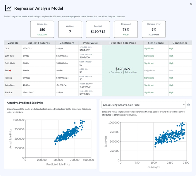
Every regression run reports quality indicators. Two describe the model as a whole; two describe each individual unit rate.
Model-level indicators
R-squared tells you what share of the price variation the model successfully explains. Higher is better.
| R² | Rating |
|---|---|
| ≥ 0.85 | Excellent |
| 0.70 – 0.85 | Good |
| 0.50 – 0.70 | Acceptable |
| 0.30 – 0.50 | Weak |
| < 0.30 | Poor |
Standard error describes the typical size of the model’s prediction errors, expressed as a percentage of price. Lower is better.
| Standard error | Rating |
|---|---|
| < 5% | Excellent |
| 5% – 8% | Good |
| 8% – 12% | Acceptable |
| 12% – 15% | Weak |
| > 15% | Poor |
If the model as a whole falls into the weaker bands, Toolkit flags it so you know the results for that order should be treated with caution.
Per-feature indicators
P-value tells you whether an individual rate is statistically meaningful or could just be noise. A p-value below 0.05 is considered significant; you’ll see the rate labeled Significant or Insignificant. An insignificant rate means the data isn’t strong enough to stand behind that specific number.
Confidence interval is the range the true rate most likely falls within (at 95% confidence). A narrow range means a precise estimate. A range that crosses zero — for example, a site-size rate from -$20,000 to $120,000 — means the model can’t even tell you whether the feature adds or subtracts value. That will always pair with a high p-value.
What to do with a weak rate. When a feature’s rate isn’t statistically defensible, Toolkit flags that row rather than presenting a number it can’t support, and it falls back to sensitivity analysis for that feature. You’re always free to review the rate and override it with your own judgment.
Sensitivity Analysis
What it is
Sensitivity analysis is the fallback for features that regression can’t handle well — for example, features that don’t have enough clean data in the pool, or where you want the rate to reflect how the comps actually reconcile against your subject. Rather than deriving a rate from a large sample, it finds the single adjustment rate that makes your comparable sales agree with one another as closely as possible.
How it works
1. It tests a range of possible rates. For a given feature, Toolkit steps through a wide range of candidate unit rates — for GLA, for instance, starting at $1 per square foot and incrementing up to $200.
2. It adjusts the comps at each rate. For every candidate rate, it adjusts each comparable sale for its difference from the subject on that feature. Note that the comp sale price used here is already adjusted for date of sale, so the feature adjustment builds on top of that date-adjusted figure:
Adjusted Sale Price = Date-Adjusted Comp Sale Price + (Feature Difference × Adjustment Rate)
3. It picks the rate that tightens the comps the most. After adjustment, it measures the spread — the gap between the highest and lowest adjusted sale prices. The rate that produces the smallest spread is the one it selects, because that rate does the best job of reconciling your comps into a tight, consistent range.
How to assess the results
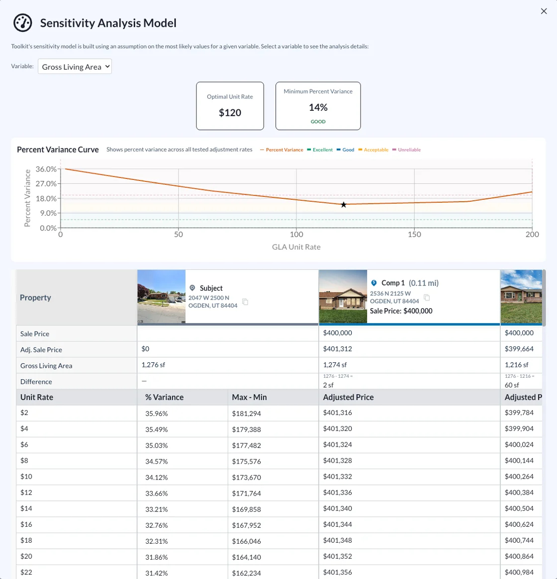
Sensitivity quality is measured by how tight that spread is, expressed as a percentage of the lowest adjusted sale price (the percent variance). A small percentage means the selected rate reconciled the comps well; a large one means even the best available rate couldn’t bring them into agreement — a sign the feature doesn’t have a clean, consistent pricing signal in this comp set.
| Percent variance | Rating |
|---|---|
| < 5% | Excellent |
| 5% – 10% | Good |
| 10% – 15% | Acceptable |
| > 15% | Poor |
Anything above 15% is flagged as unreliable. At that level the adjusted sale prices are still too spread out to treat the derived rate as a defensible adjustment, and you should apply your own judgment.
How the two work together
Regression is the primary method — it draws on a large sample and reports the fullest set of diagnostics. Sensitivity analysis supports it, stepping in for individual features where regression can’t produce a defensible rate. For any feature, Toolkit uses the reliable regression rate if it has one, falls back to the reliable sensitivity rate if it doesn’t, and otherwise leaves the rate for you to set. In every case the underlying statistics are shown alongside the rate, and you retain full control to override any adjustment.
Note: the supporting statistics are viewable on the Adjustments page within Toolkit.
